 This is an excerpt from the
 Regresión Lineal
%matplotlib inline
import matplotlib.pyplot as plt
import seaborn as sns; sns.set()
import numpy as np
Regresión Lineal Simple
A straight-line fit is a model of the form $$ y = ax + b $$ where $a$ is commonly known as the slope, and $b$ is commonly known as the intercept.
rng = np.random.RandomState(1)
x = 10 * rng.rand(50)
y = 2 * x - 5 + rng.randn(50)
plt.scatter(x, y);

from sklearn.linear_model import LinearRegression
model = LinearRegression(fit_intercept=True)

model.fit(x[:, np.newaxis], y)

xfit = np.linspace(0, 10, 1000)
yfit = model.predict(xfit[:, np.newaxis])

plt.scatter(x, y)
plt.plot(xfit, yfit);

print("Model slope:    ", model.coef_[0])
print("Model intercept:", model.intercept_)
rng = np.random.RandomState(1)
X = 10 * rng.rand(100, 3)
y = 0.5 + np.dot(X, [1.5, -2., 1.])

model.fit(X, y)
print(model.intercept_)
print(model.coef_)
Regresión usando funciones base
One trick you can use to adapt linear regression to nonlinear relationships between variables is to transform the data according to basis functions.
We have seen one version of this before, in the PolynomialRegression pipeline used in Hyperparameters and Model Validation and Feature Engineering.
The idea is to take our multidimensional linear model:
$$
y = a_0 + a_1 x_1 + a_2 x_2 + a_3 x_3 + \cdots
$$
and build the $x_1, x_2, x_3,$ and so on, from our single-dimensional input $x$.
That is, we let $x_n = f_n(x)$, where $f_n()$ is some function that transforms our data.
For example, if $f_n(x) = x^n$, our model becomes a polynomial regression: $$ y = a_0 + a_1 x + a_2 x^2 + a_3 x^3 + \cdots $$ Notice that this is still a linear model—the linearity refers to the fact that the coefficients $a_n$ never multiply or divide each other. What we have effectively done is taken our one-dimensional $x$ values and projected them into a higher dimension, so that a linear fit can fit more complicated relationships between $x$ and $y$.
Bases Polinomiales
from sklearn.preprocessing import PolynomialFeatures
x = np.array([2, 3, 4])
poly = PolynomialFeatures(3, include_bias=False)
poly.fit_transform(x[:, None])
from sklearn.pipeline import make_pipeline
poly_model = make_pipeline(PolynomialFeatures(7),
                           LinearRegression())
rng = np.random.RandomState(1)
x = 10 * rng.rand(50)
y = np.sin(x) + 0.1 * rng.randn(50)

poly_model.fit(x[:, np.newaxis], y)
yfit = poly_model.predict(xfit[:, np.newaxis])

plt.scatter(x, y)
plt.plot(xfit, yfit);

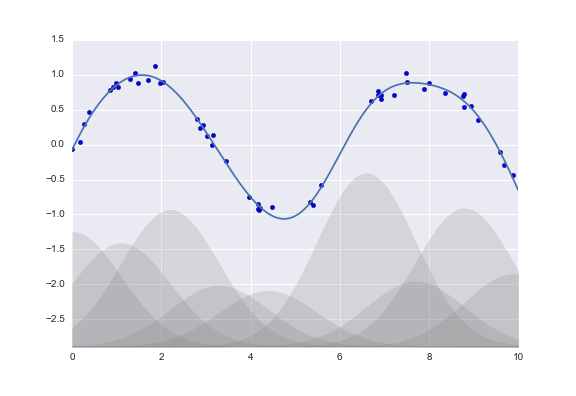
Bases Gaussianas
from sklearn.base import BaseEstimator, TransformerMixin

class GaussianFeatures(BaseEstimator, TransformerMixin):
    """Uniformly spaced Gaussian features for one-dimensional input"""

    def __init__(self, N, width_factor=2.0):
        self.N = N
        self.width_factor = width_factor

    @staticmethod
    def _gauss_basis(x, y, width, axis=None):
        arg = (x - y) / width
        return np.exp(-0.5 * np.sum(arg ** 2, axis))

    def fit(self, X, y=None):
        # create N centers spread along the data range
        self.centers_ = np.linspace(X.min(), X.max(), self.N)
        self.width_ = self.width_factor * (self.centers_[1] - self.centers_[0])
        return self

    def transform(self, X):
        return self._gauss_basis(X[:, :, np.newaxis], self.centers_,
                                 self.width_, axis=1)

gauss_model = make_pipeline(GaussianFeatures(20),
                            LinearRegression())
gauss_model.fit(x[:, np.newaxis], y)
yfit = gauss_model.predict(xfit[:, np.newaxis])

plt.scatter(x, y)
plt.plot(xfit, yfit)
plt.xlim(0, 10);

Regularización
model = make_pipeline(GaussianFeatures(30),
                      LinearRegression())
model.fit(x[:, np.newaxis], y)

plt.scatter(x, y)
plt.plot(xfit, model.predict(xfit[:, np.newaxis]))

plt.xlim(0, 10)
plt.ylim(-1.5, 1.5);

def basis_plot(model, title=None):
    fig, ax = plt.subplots(2, sharex=True)
    model.fit(x[:, np.newaxis], y)
    ax[0].scatter(x, y)
    ax[0].plot(xfit, model.predict(xfit[:, np.newaxis]))
    ax[0].set(xlabel='x', ylabel='y', ylim=(-1.5, 1.5))

    if title:
        ax[0].set_title(title)

    ax[1].plot(model.steps[0][1].centers_,
               model.steps[1][1].coef_)
    ax[1].set(xlabel='basis location',
              ylabel='coefficient',
              xlim=(0, 10))

model = make_pipeline(GaussianFeatures(30), LinearRegression())
basis_plot(model)

Regularización $L_2$ (regresión de cresta)
from sklearn.linear_model import Ridge
model = make_pipeline(GaussianFeatures(30), Ridge(alpha=0.1))
basis_plot(model, title='Ridge Regression')

Regularización $L_1$ (regresión de lasso)
from sklearn.linear_model import Lasso
model = make_pipeline(GaussianFeatures(30), Lasso(alpha=0.001))
basis_plot(model, title='Lasso Regression')

Ejemplo: Predicción de tráfico
# !curl -o FremontBridge.csv https://data.seattle.gov/api/views/65db-xm6k/rows.csv?accessType=DOWNLOAD
import pandas as pd
counts = pd.read_csv('FremontBridge.csv', index_col='Date', parse_dates=True)
weather = pd.read_csv('data/BicycleWeather.csv', index_col='DATE', parse_dates=True)
daily = counts.resample('d').sum()
daily['Total'] = daily.sum(axis=1)
daily = daily[['Total']] # remove other columns
days = ['Mon', 'Tue', 'Wed', 'Thu', 'Fri', 'Sat', 'Sun']
for i in range(7):
    daily[days[i]] = (daily.index.dayofweek == i).astype(float)
from pandas.tseries.holiday import USFederalHolidayCalendar
cal = USFederalHolidayCalendar()
holidays = cal.holidays('2012', '2016')
daily = daily.join(pd.Series(1, index=holidays, name='holiday'))
daily['holiday'].fillna(0, inplace=True)
def hours_of_daylight(date, axis=23.44, latitude=47.61):
    """Compute the hours of daylight for the given date"""
    days = (date - pd.datetime(2000, 12, 21)).days
    m = (1. - np.tan(np.radians(latitude))
         * np.tan(np.radians(axis) * np.cos(days * 2 * np.pi / 365.25)))
    return 24. * np.degrees(np.arccos(1 - np.clip(m, 0, 2))) / 180.

daily['daylight_hrs'] = list(map(hours_of_daylight, daily.index))
daily[['daylight_hrs']].plot()
plt.ylim(8, 17)

# temperatures are in 1/10 deg C; convert to C
weather['TMIN'] /= 10
weather['TMAX'] /= 10
weather['Temp (C)'] = 0.5 * (weather['TMIN'] + weather['TMAX'])

# precip is in 1/10 mm; convert to inches
weather['PRCP'] /= 254
weather['dry day'] = (weather['PRCP'] == 0).astype(int)

daily = daily.join(weather[['PRCP', 'Temp (C)', 'dry day']])
daily['annual'] = (daily.index - daily.index[0]).days / 365.
daily.head()
# Drop any rows with null values
daily.dropna(axis=0, how='any', inplace=True)

column_names = ['Mon', 'Tue', 'Wed', 'Thu', 'Fri', 'Sat', 'Sun', 'holiday',
                'daylight_hrs', 'PRCP', 'dry day', 'Temp (C)', 'annual']
X = daily[column_names]
y = daily['Total']

model = LinearRegression(fit_intercept=False)
model.fit(X, y)
daily['predicted'] = model.predict(X)
daily[['Total', 'predicted']].plot(alpha=0.5);

params = pd.Series(model.coef_, index=X.columns)
params
from sklearn.utils import resample
np.random.seed(1)
err = np.std([model.fit(*resample(X, y)).coef_
              for i in range(1000)], 0)
print(pd.DataFrame({'effect': params.round(0),
                    'error': err.round(0)}))