Clasificacion usando Naive Bayes

< Ingeniería de Atributos | Contenido | Regresión Lineal >

Clasificación Bayesiana¶

Naive Bayes classifiers are built on Bayesian classification methods. These rely on Bayes's theorem, which is an equation describing the relationship of conditional probabilities of statistical quantities. In Bayesian classification, we're interested in finding the probability of a label given some observed features, which we can write as $P(L~|~{\rm features})$. Bayes's theorem tells us how to express this in terms of quantities we can compute more directly:

$$ P(L~|~{\rm features}) = \frac{P({\rm features}~|~L)P(L)}{P({\rm features})} $$

If we are trying to decide between two labels—let's call them $L_1$ and $L_2$—then one way to make this decision is to compute the ratio of the posterior probabilities for each label:

$$ \frac{P(L_1~|~{\rm features})}{P(L_2~|~{\rm features})} = \frac{P({\rm features}~|~L_1)}{P({\rm features}~|~L_2)}\frac{P(L_1)}{P(L_2)} $$

In [1]:

%matplotlib inline
import numpy as np
import matplotlib.pyplot as plt
import seaborn as sns; sns.set()

Bayes Gaussiano¶

In [2]:

from sklearn.datasets import make_blobs
X, y = make_blobs(100, 2, centers=2, random_state=2, cluster_std=1.5)
plt.scatter(X[:, 0], X[:, 1], c=y, s=50, cmap='RdBu');

(run code in Appendix to generate image) figure source in Appendix

In [3]:

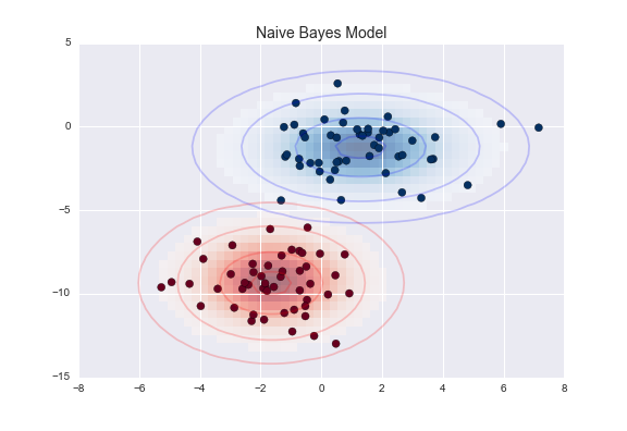
from sklearn.naive_bayes import GaussianNB
model = GaussianNB()
model.fit(X, y);

In [4]:

rng = np.random.RandomState(0)
Xnew = [-6, -14] + [14, 18] * rng.rand(2000, 2)
ynew = model.predict(Xnew)

In [5]:

plt.scatter(X[:, 0], X[:, 1], c=y, s=50, cmap='RdBu')
lim = plt.axis()
plt.scatter(Xnew[:, 0], Xnew[:, 1], c=ynew, s=20, cmap='RdBu', alpha=0.1)
plt.axis(lim);

In [6]:

yprob = model.predict_proba(Xnew)
yprob[-8:].round(2)

Out[6]:

array([[ 0.89,  0.11],
       [ 1.  ,  0.  ],
       [ 1.  ,  0.  ],
       [ 1.  ,  0.  ],
       [ 1.  ,  0.  ],
       [ 1.  ,  0.  ],
       [ 0.  ,  1.  ],
       [ 0.15,  0.85]])

Bayes Multinomial¶

Ejemplo: Clasificación de texto¶

In [7]:

from sklearn.datasets import fetch_20newsgroups

data = fetch_20newsgroups()
data.target_names

Out[7]:

['alt.atheism',
 'comp.graphics',
 'comp.os.ms-windows.misc',
 'comp.sys.ibm.pc.hardware',
 'comp.sys.mac.hardware',
 'comp.windows.x',
 'misc.forsale',
 'rec.autos',
 'rec.motorcycles',
 'rec.sport.baseball',
 'rec.sport.hockey',
 'sci.crypt',
 'sci.electronics',
 'sci.med',
 'sci.space',
 'soc.religion.christian',
 'talk.politics.guns',
 'talk.politics.mideast',
 'talk.politics.misc',
 'talk.religion.misc']

In [8]:

categories = ['talk.religion.misc', 'soc.religion.christian',
              'sci.space', 'comp.graphics']
train = fetch_20newsgroups(subset='train', categories=categories)
test = fetch_20newsgroups(subset='test', categories=categories)

In [9]:

print(train.data[5])

From: dmcgee@uluhe.soest.hawaii.edu (Don McGee)
Subject: Federal Hearing
Originator: dmcgee@uluhe
Organization: School of Ocean and Earth Science and Technology
Distribution: usa
Lines: 10

Fact or rumor....?  Madalyn Murray O'Hare an atheist who eliminated the
use of the bible reading and prayer in public schools 15 years ago is now
going to appear before the FCC with a petition to stop the reading of the
Gospel on the airways of America.  And she is also campaigning to remove
Christmas programs, songs, etc from the public schools.  If it is true
then mail to Federal Communications Commission 1919 H Street Washington DC
20054 expressing your opposition to her request.  Reference Petition number

2493.

In [10]:

from sklearn.feature_extraction.text import TfidfVectorizer
from sklearn.naive_bayes import MultinomialNB
from sklearn.pipeline import make_pipeline

model = make_pipeline(TfidfVectorizer(), MultinomialNB())

In [11]:

model.fit(train.data, train.target)
labels = model.predict(test.data)

In [12]:

from sklearn.metrics import confusion_matrix
mat = confusion_matrix(test.target, labels)
sns.heatmap(mat.T, square=True, annot=True, fmt='d', cbar=False,
            xticklabels=train.target_names, yticklabels=train.target_names)
plt.xlabel('true label')
plt.ylabel('predicted label');

In [13]:

def predict_category(s, train=train, model=model):
    pred = model.predict([s])
    return train.target_names[pred[0]]

In [14]:

predict_category('sending a payload to the ISS')

Out[14]:

'sci.space'

In [15]:

predict_category('discussing islam vs atheism')

Out[15]:

'soc.religion.christian'

In [16]:

predict_category('determining the screen resolution')

Out[16]:

'comp.graphics'

Cuando usar Naive Bayes¶

Because naive Bayesian classifiers make such stringent assumptions about data, they will generally not perform as well as a more complicated model. That said, they have several advantages:

They are extremely fast for both training and prediction
They provide straightforward probabilistic prediction
They are often very easily interpretable
They have very few (if any) tunable parameters

These advantages mean a naive Bayesian classifier is often a good choice as an initial baseline classification. If it performs suitably, then congratulations: you have a very fast, very interpretable classifier for your problem. If it does not perform well, then you can begin exploring more sophisticated models, with some baseline knowledge of how well they should perform.

Naive Bayes classifiers tend to perform especially well in one of the following situations:

When the naive assumptions actually match the data (very rare in practice)
For very well-separated categories, when model complexity is less important
For very high-dimensional data, when model complexity is less important

The last two points seem distinct, but they actually are related: as the dimension of a dataset grows, it is much less likely for any two points to be found close together (after all, they must be close in every single dimension to be close overall). This means that clusters in high dimensions tend to be more separated, on average, than clusters in low dimensions, assuming the new dimensions actually add information. For this reason, simplistic classifiers like naive Bayes tend to work as well or better than more complicated classifiers as the dimensionality grows: once you have enough data, even a simple model can be very powerful.

< Ingeniería de Atributos | Contenido | Regresión Lineal >