 This is an excerpt from the
 Hiperparámetros y validación de modelos
Validación de modelos
Como no hacer una validación del modelo
from sklearn.datasets import load_iris
iris = load_iris()
X = iris.data
y = iris.target
from sklearn.neighbors import KNeighborsClassifier
model = KNeighborsClassifier(n_neighbors=1)
model.fit(X, y)
y_model = model.predict(X)
from sklearn.metrics import accuracy_score
accuracy_score(y, y_model)
Forma correcta para la validación del modelo: conjuntos de prueba
from sklearn.cross_validation import train_test_split
# split the data with 50% in each set
X1, X2, y1, y2 = train_test_split(X, y, random_state=0,
                                  train_size=0.5)

# fit the model on one set of data
model.fit(X1, y1)

# evaluate the model on the second set of data
y2_model = model.predict(X2)
accuracy_score(y2, y2_model)
Validación cuzada de modelos (cross-validation)
y2_model = model.fit(X1, y1).predict(X2)
y1_model = model.fit(X2, y2).predict(X1)
accuracy_score(y1, y1_model), accuracy_score(y2, y2_model)
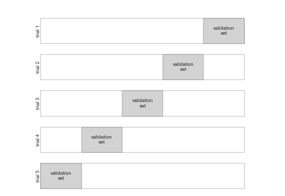
here is a visual depiction of five-fold cross-validation:
from sklearn.cross_validation import cross_val_score
cross_val_score(model, X, y, cv=5)
from sklearn.cross_validation import LeaveOneOut
scores = cross_val_score(model, X, y, cv=LeaveOneOut(len(X)))
scores
scores.mean()
Other cross-validation schemes can be used similarly.
For a description of what is available in Scikit-Learn, use IPython to explore the sklearn.cross_validation submodule, or take a look at Scikit-Learn's online cross-validation documentation.
Selección del mejor modelo
Of core importance is the following question: if our estimator is underperforming, how should we move forward? There are several possible answers:
- Use a more complicated/more flexible model
- Use a less complicated/less flexible model
- Gather more training samples
- Gather more data to add features to each sample
The answer to this question is often counter-intuitive. In particular, sometimes using a more complicated model will give worse results, and adding more training samples may not improve your results! The ability to determine what steps will improve your model is what separates the successful machine learning practitioners from the unsuccessful.
Compensando entre la varianza y la tendencia
Fundamentally, the question of "the best model" is about finding a sweet spot in the tradeoff between bias and variance. Consider the following figure, which presents two regression fits to the same dataset:
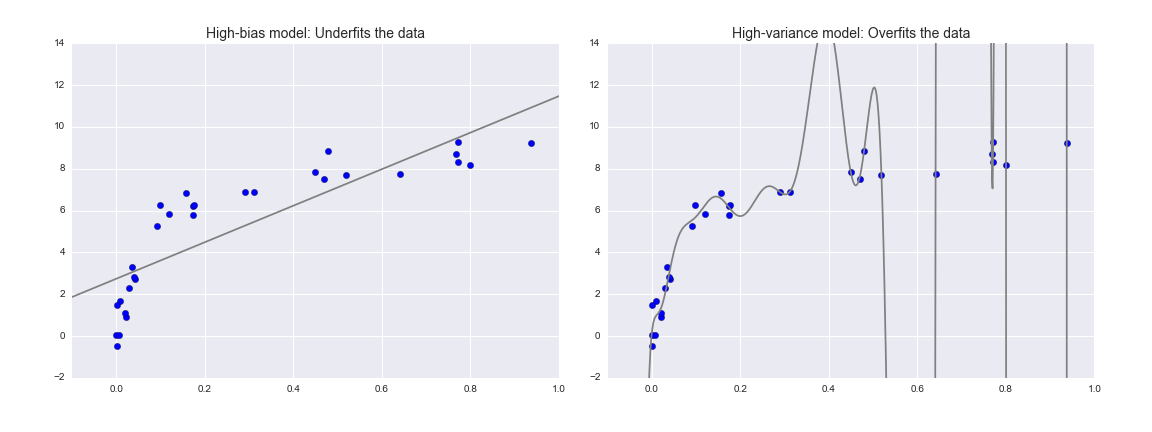
It is clear that neither of these models is a particularly good fit to the data, but they fail in different ways.
The model on the left attempts to find a straight-line fit through the data. Because the data are intrinsically more complicated than a straight line, the straight-line model will never be able to describe this dataset well. Such a model is said to underfit the data: that is, it does not have enough model flexibility to suitably account for all the features in the data; another way of saying this is that the model has high bias.
The model on the right attempts to fit a high-order polynomial through the data. Here the model fit has enough flexibility to nearly perfectly account for the fine features in the data, but even though it very accurately describes the training data, its precise form seems to be more reflective of the particular noise properties of the data rather than the intrinsic properties of whatever process generated that data. Such a model is said to overfit the data: that is, it has so much model flexibility that the model ends up accounting for random errors as well as the underlying data distribution; another way of saying this is that the model has high variance.
To look at this in another light, consider what happens if we use these two models to predict the y-value for some new data. In the following diagrams, the red/lighter points indicate data that is omitted from the training set:
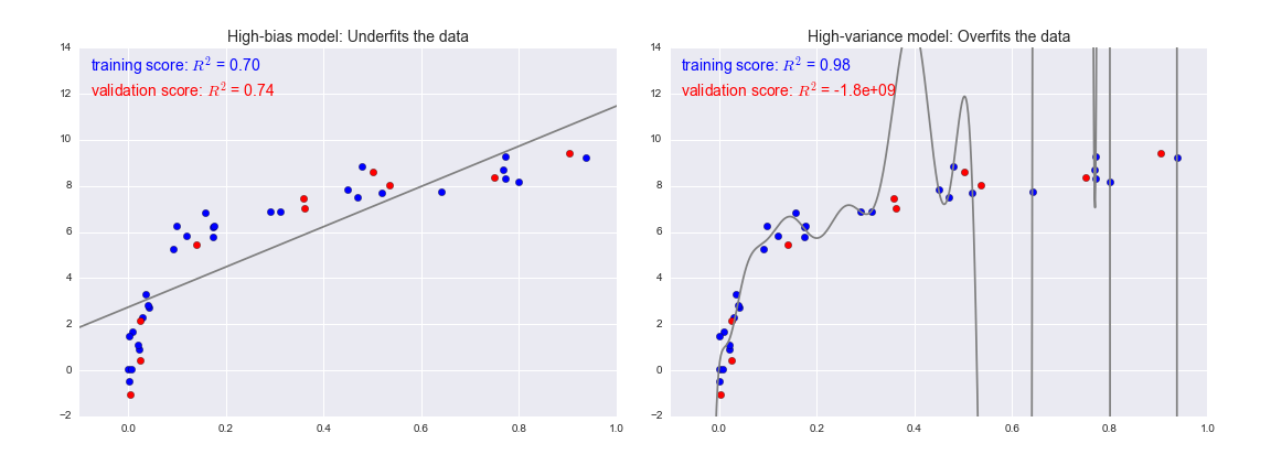
The score here is the $R^2$ score, or coefficient of determination, which measures how well a model performs relative to a simple mean of the target values. $R^2=1$ indicates a perfect match, $R^2=0$ indicates the model does no better than simply taking the mean of the data, and negative values mean even worse models. From the scores associated with these two models, we can make an observation that holds more generally:
- For high-bias models, the performance of the model on the validation set is similar to the performance on the training set.
- For high-variance models, the performance of the model on the validation set is far worse than the performance on the training set.
If we imagine that we have some ability to tune the model complexity, we would expect the training score and validation score to behave as illustrated in the following figure:
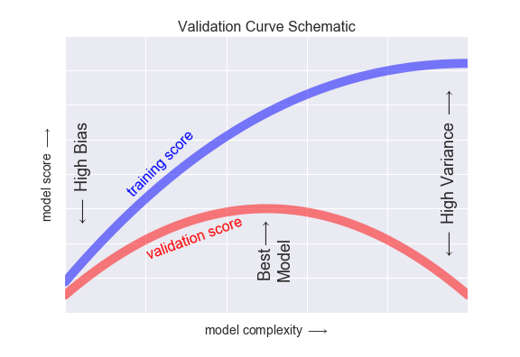
The diagram shown here is often called a validation curve, and we see the following essential features:
- The training score is everywhere higher than the validation score. This is generally the case: the model will be a better fit to data it has seen than to data it has not seen.
- For very low model complexity (a high-bias model), the training data is under-fit, which means that the model is a poor predictor both for the training data and for any previously unseen data.
- For very high model complexity (a high-variance model), the training data is over-fit, which means that the model predicts the training data very well, but fails for any previously unseen data.
- For some intermediate value, the validation curve has a maximum. This level of complexity indicates a suitable trade-off between bias and variance.
The means of tuning the model complexity varies from model to model; when we discuss individual models in depth in later sections, we will see how each model allows for such tuning.
Curvas de validación en Scikit-Learn
Let's look at an example of using cross-validation to compute the validation curve for a class of models. Here we will use a polynomial regression model: this is a generalized linear model in which the degree of the polynomial is a tunable parameter. For example, a degree-1 polynomial fits a straight line to the data; for model parameters $a$ and $b$:
$$ y = ax + b $$A degree-3 polynomial fits a cubic curve to the data; for model parameters $a, b, c, d$:
$$ y = ax^3 + bx^2 + cx + d $$We can generalize this to any number of polynomial features. In Scikit-Learn, we can implement this with a simple linear regression combined with the polynomial preprocessor. We will use a pipeline to string these operations together (we will discuss polynomial features and pipelines more fully in Feature Engineering):
from sklearn.preprocessing import PolynomialFeatures
from sklearn.linear_model import LinearRegression
from sklearn.pipeline import make_pipeline

def PolynomialRegression(degree=2, **kwargs):
    return make_pipeline(PolynomialFeatures(degree),
                         LinearRegression(**kwargs))
import numpy as np

def make_data(N, err=1.0, rseed=1):
    # randomly sample the data
    rng = np.random.RandomState(rseed)
    X = rng.rand(N, 1) ** 2
    y = 10 - 1. / (X.ravel() + 0.1)
    if err > 0:
        y += err * rng.randn(N)
    return X, y

X, y = make_data(40)
%matplotlib inline
import matplotlib.pyplot as plt
import seaborn; seaborn.set()  # plot formatting

X_test = np.linspace(-0.1, 1.1, 500)[:, None]

plt.scatter(X.ravel(), y, color='black')
axis = plt.axis()
for degree in [1, 3, 5]:
    y_test = PolynomialRegression(degree).fit(X, y).predict(X_test)
    plt.plot(X_test.ravel(), y_test, label='degree={0}'.format(degree))
plt.xlim(-0.1, 1.0)
plt.ylim(-2, 12)
plt.legend(loc='best');

from sklearn.learning_curve import validation_curve
degree = np.arange(0, 21)
train_score, val_score = validation_curve(PolynomialRegression(), X, y,
                                          'polynomialfeatures__degree', degree, cv=7)

plt.plot(degree, np.median(train_score, 1), color='blue', label='training score')
plt.plot(degree, np.median(val_score, 1), color='red', label='validation score')
plt.legend(loc='best')
plt.ylim(0, 1)
plt.xlabel('degree')
plt.ylabel('score');

plt.scatter(X.ravel(), y)
lim = plt.axis()
y_test = PolynomialRegression(3).fit(X, y).predict(X_test)
plt.plot(X_test.ravel(), y_test);
plt.axis(lim);

Curvas de aprendizaje
X2, y2 = make_data(200)
plt.scatter(X2.ravel(), y2);

degree = np.arange(21)
train_score2, val_score2 = validation_curve(PolynomialRegression(), X2, y2,
                                            'polynomialfeatures__degree', degree, cv=7)

plt.plot(degree, np.median(train_score2, 1), color='blue', label='training score')
plt.plot(degree, np.median(val_score2, 1), color='red', label='validation score')
plt.plot(degree, np.median(train_score, 1), color='blue', alpha=0.3, linestyle='dashed')
plt.plot(degree, np.median(val_score, 1), color='red', alpha=0.3, linestyle='dashed')
plt.legend(loc='lower center')
plt.ylim(0, 1)
plt.xlabel('degree')
plt.ylabel('score');

The solid lines show the new results, while the fainter dashed lines show the results of the previous smaller dataset. It is clear from the validation curve that the larger dataset can support a much more complicated model: the peak here is probably around a degree of 6, but even a degree-20 model is not seriously over-fitting the data—the validation and training scores remain very close.
Thus we see that the behavior of the validation curve has not one but two important inputs: the model complexity and the number of training points. It is often useful to to explore the behavior of the model as a function of the number of training points, which we can do by using increasingly larger subsets of the data to fit our model. A plot of the training/validation score with respect to the size of the training set is known as a learning curve.
The general behavior we would expect from a learning curve is this:
- A model of a given complexity will overfit a small dataset: this means the training score will be relatively high, while the validation score will be relatively low.
- A model of a given complexity will underfit a large dataset: this means that the training score will decrease, but the validation score will increase.
- A model will never, except by chance, give a better score to the validation set than the training set: this means the curves should keep getting closer together but never cross.
With these features in mind, we would expect a learning curve to look qualitatively like that shown in the following figure:
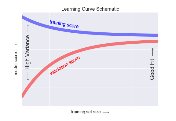
The notable feature of the learning curve is the convergence to a particular score as the number of training samples grows. In particular, once you have enough points that a particular model has converged, adding more training data will not help you! The only way to increase model performance in this case is to use another (often more complex) model.
Curvas de aprendizaje en Scikit-Learn
Scikit-Learn offers a convenient utility for computing such learning curves from your models; here we will compute a learning curve for our original dataset with a second-order polynomial model and a ninth-order polynomial:
from sklearn.learning_curve import learning_curve

fig, ax = plt.subplots(1, 2, figsize=(16, 6))
fig.subplots_adjust(left=0.0625, right=0.95, wspace=0.1)

for i, degree in enumerate([2, 9]):
    N, train_lc, val_lc = learning_curve(PolynomialRegression(degree),
                                         X, y, cv=7,
                                         train_sizes=np.linspace(0.3, 1, 25))

    ax[i].plot(N, np.mean(train_lc, 1), color='blue', label='training score')
    ax[i].plot(N, np.mean(val_lc, 1), color='red', label='validation score')
    ax[i].hlines(np.mean([train_lc[-1], val_lc[-1]]), N[0], N[-1],
                 color='gray', linestyle='dashed')

    ax[i].set_ylim(0, 1)
    ax[i].set_xlim(N[0], N[-1])
    ax[i].set_xlabel('training size')
    ax[i].set_ylabel('score')
    ax[i].set_title('degree = {0}'.format(degree), size=14)
    ax[i].legend(loc='best')

Validación en la práctica: Grid Search
The preceding discussion is meant to give you some intuition into the trade-off between bias and variance, and its dependence on model complexity and training set size. In practice, models generally have more than one knob to turn, and thus plots of validation and learning curves change from lines to multi-dimensional surfaces. In these cases, such visualizations are difficult and we would rather simply find the particular model that maximizes the validation score.
Scikit-Learn provides automated tools to do this in the grid search module.
Here is an example of using grid search to find the optimal polynomial model.
We will explore a three-dimensional grid of model features; namely the polynomial degree, the flag telling us whether to fit the intercept, and the flag telling us whether to normalize the problem.
This can be set up using Scikit-Learn's GridSearchCV meta-estimator:
from sklearn.grid_search import GridSearchCV

param_grid = {'polynomialfeatures__degree': np.arange(21),
              'linearregression__fit_intercept': [True, False],
              'linearregression__normalize': [True, False]}

grid = GridSearchCV(PolynomialRegression(), param_grid, cv=7)
grid.fit(X, y);
grid.best_params_
model = grid.best_estimator_

plt.scatter(X.ravel(), y)
lim = plt.axis()
y_test = model.fit(X, y).predict(X_test)
plt.plot(X_test.ravel(), y_test, hold=True);
plt.axis(lim);

Summary
En ésta sección exploramos el concepto de validación de modelo y optimización de hiperparámetros, enfocados en los aspectos de tendencia y varianza de los datos y su efecto en el modelado. El uso de conjuntos de validación o validación cruzada son fundamentales para obtener los mejores parámetros y evitar el efecto de un sobre ajuste del modelo, lo cual permite explorar el uso de modelos más complejos o flexibles.