< ¿Qué es Machine Learning? | Contenido | Hiperparámetros y validación de modelos >

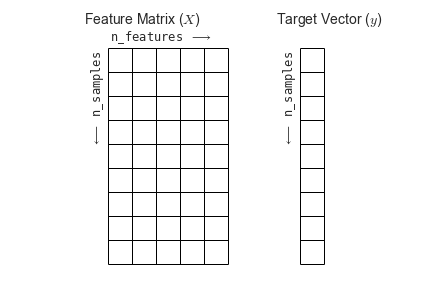
Representación de datos en Scikit-Learn¶

Datos como tablas¶

In [1]:

import seaborn as sns
iris = sns.load_dataset('iris')
iris.head()

Out[1]:

	sepal_length	sepal_width	petal_length	petal_width	species
0	5.1	3.5	1.4	0.2	setosa
1	4.9	3.0	1.4	0.2	setosa
2	4.7	3.2	1.3	0.2	setosa
3	4.6	3.1	1.5	0.2	setosa
4	5.0	3.6	1.4	0.2	setosa

Matriz de atributos¶

Vector de objetivos¶

In [2]:

%matplotlib inline
import seaborn as sns; sns.set()
sns.pairplot(iris, hue='species', size=1.5);

In [3]:

X_iris = iris.drop('species', axis=1)
X_iris.shape

Out[3]:

(150, 4)

In [4]:

y_iris = iris['species']
y_iris.shape

Out[4]:

(150,)

figure source in Appendix

API de Estimadores de Scikit-Learn¶

Básicos de la API¶

Most commonly, the steps in using the Scikit-Learn estimator API are as follows (we will step through a handful of detailed examples in the sections that follow).

Choose a class of model by importing the appropriate estimator class from Scikit-Learn.
Choose model hyperparameters by instantiating this class with desired values.
Arrange data into a features matrix and target vector following the discussion above.
Fit the model to your data by calling the fit() method of the model instance.
Apply the Model to new data:
- For supervised learning, often we predict labels for unknown data using the predict() method.
- For unsupervised learning, we often transform or infer properties of the data using the transform() or predict() method.

We will now step through several simple examples of applying supervised and unsupervised learning methods.

Ejemplo de aprendizaje supervisado: regresión lineal simple¶

In [5]:

import matplotlib.pyplot as plt
import numpy as np

rng = np.random.RandomState(42)
x = 10 * rng.rand(50)
y = 2 * x - 1 + rng.randn(50)
plt.scatter(x, y);

1. Elegir una clase de model¶

In [6]:

from sklearn.linear_model import LinearRegression

2. Elegir los hiperparametros del model¶

In [7]:

model = LinearRegression(fit_intercept=True)
model

Out[7]:

LinearRegression(copy_X=True, fit_intercept=True, n_jobs=1, normalize=False)

3. Acomodar los datos en una matriz de atributos y un vector de objetivos¶

In [8]:

X = x[:, np.newaxis]
X.shape

Out[8]:

(50, 1)

4. Ajustar el modelo a los datos¶

In [9]:

model.fit(X, y)

Out[9]:

LinearRegression(copy_X=True, fit_intercept=True, n_jobs=1, normalize=False)

In [10]:

model.coef_

Out[10]:

array([ 1.9776566])

In [11]:

model.intercept_

Out[11]:

-0.90331072553111635

5. Predicción usando el modelo con datos nuevos¶

In [12]:

xfit = np.linspace(-1, 11)

In [13]:

Xfit = xfit[:, np.newaxis]
yfit = model.predict(Xfit)

In [14]:

plt.scatter(x, y)
plt.plot(xfit, yfit);

Ejemplo de aprendizaje supervisado: clasificación del conjunto de Iris¶

In [15]:

from sklearn.cross_validation import train_test_split
Xtrain, Xtest, ytrain, ytest = train_test_split(X_iris, y_iris,
                                                random_state=1)

In [16]:

from sklearn.naive_bayes import GaussianNB # 1. choose model class
model = GaussianNB()                       # 2. instantiate model
model.fit(Xtrain, ytrain)                  # 3. fit model to data
y_model = model.predict(Xtest)             # 4. predict on new data

In [17]:

from sklearn.metrics import accuracy_score
accuracy_score(ytest, y_model)

Out[17]:

0.97368421052631582

Ejemplo de aprendizaje no supervisado: dimensionalidad del conjunto de Iris¶

In [18]:

from sklearn.decomposition import PCA  # 1. Choose the model class
model = PCA(n_components=2)            # 2. Instantiate the model with hyperparameters
model.fit(X_iris)                      # 3. Fit to data. Notice y is not specified!
X_2D = model.transform(X_iris)         # 4. Transform the data to two dimensions

In [19]:

iris['PCA1'] = X_2D[:, 0]
iris['PCA2'] = X_2D[:, 1]
sns.lmplot("PCA1", "PCA2", hue='species', data=iris, fit_reg=False);

Aprendizaje no superviado: acumulación del conjunto de Iris¶

In [20]:

from sklearn.mixture import GMM      # 1. Choose the model class
model = GMM(n_components=3,
            covariance_type='full')  # 2. Instantiate the model with hyperparameters
model.fit(X_iris)                    # 3. Fit to data. Notice y is not specified!
y_gmm = model.predict(X_iris)        # 4. Determine cluster labels

In [21]:

iris['cluster'] = y_gmm
sns.lmplot("PCA1", "PCA2", data=iris, hue='species',
           col='cluster', fit_reg=False);

Aplicación: Digitos escritos a mano¶

Cargando y visualizando los datos¶

In [22]:

from sklearn.datasets import load_digits
digits = load_digits()
digits.images.shape

Out[22]:

(1797, 8, 8)

In [23]:

import matplotlib.pyplot as plt

fig, axes = plt.subplots(10, 10, figsize=(8, 8),
                         subplot_kw={'xticks':[], 'yticks':[]},
                         gridspec_kw=dict(hspace=0.1, wspace=0.1))

for i, ax in enumerate(axes.flat):
    ax.imshow(digits.images[i], cmap='binary', interpolation='nearest')
    ax.text(0.05, 0.05, str(digits.target[i]),
            transform=ax.transAxes, color='green')

In [24]:

X = digits.data
X.shape

Out[24]:

(1797, 64)

In [25]:

y = digits.target
y.shape

Out[25]:

(1797,)

Aprendizaje no supervisado: Reducción de dimensionalidad¶

In [26]:

from sklearn.manifold import Isomap
iso = Isomap(n_components=2)
iso.fit(digits.data)
data_projected = iso.transform(digits.data)
data_projected.shape

Out[26]:

(1797, 2)

In [27]:

plt.scatter(data_projected[:, 0], data_projected[:, 1], c=digits.target,
            edgecolor='none', alpha=0.5,
            cmap=plt.cm.get_cmap('spectral', 10))
plt.colorbar(label='digit label', ticks=range(10))
plt.clim(-0.5, 9.5);

Clasificación de digitos¶

In [28]:

Xtrain, Xtest, ytrain, ytest = train_test_split(X, y, random_state=0)

In [29]:

from sklearn.naive_bayes import GaussianNB
model = GaussianNB()
model.fit(Xtrain, ytrain)
y_model = model.predict(Xtest)

In [30]:

from sklearn.metrics import accuracy_score
accuracy_score(ytest, y_model)

Out[30]:

0.83333333333333337

In [31]:

from sklearn.metrics import confusion_matrix

mat = confusion_matrix(ytest, y_model)

sns.heatmap(mat, square=True, annot=True, cbar=False)
plt.xlabel('predicted value')
plt.ylabel('true value');

In [32]:

fig, axes = plt.subplots(10, 10, figsize=(8, 8),
                         subplot_kw={'xticks':[], 'yticks':[]},
                         gridspec_kw=dict(hspace=0.1, wspace=0.1))

test_images = Xtest.reshape(-1, 8, 8)

for i, ax in enumerate(axes.flat):
    ax.imshow(test_images[i], cmap='binary', interpolation='nearest')
    ax.text(0.05, 0.05, str(y_model[i]),
            transform=ax.transAxes,
            color='green' if (ytest[i] == y_model[i]) else 'red')

Resúmen¶

En esta sección hemos visto algunas de las característics esenciales de la librería Scikit-Learn y la API de estimadores. Con ésta información pueden comenzar a probar distintos de los modelos disponibles en la librería en sus datos. En las siguientes secciones veremos como elegir y validar el modelo.

< ¿Qué es Machine Learning? | Contenido | Hiperparámetros y validación de modelos >