This is an excerpt from the Python Data Science Handbook by Jake VanderPlas; Jupyter notebooks are available on GitHub.

The text is released under the CC-BY-NC-ND license, and code is released under the MIT license. If you find this content useful, please consider supporting the work by buying the book!

Agregaciones y agrupaciones

In [1]:
import numpy as np
import pandas as pd

class display(object):
    """Display HTML representation of multiple objects"""
    template = """<div style="float: left; padding: 10px;">
    <p style='font-family:"Courier New", Courier, monospace'>{0}</p>{1}
    </div>"""
    def __init__(self, *args):
        self.args = args
        
    def _repr_html_(self):
        return '\n'.join(self.template.format(a, eval(a)._repr_html_())
                         for a in self.args)
    
    def __repr__(self):
        return '\n\n'.join(a + '\n' + repr(eval(a))
                           for a in self.args)

Datos de los planetas

In [2]:
import seaborn as sns
planets = sns.load_dataset('planets')
planets.shape
Out[2]:
(1035, 6)
In [3]:
planets.head()
Out[3]:
method number orbital_period mass distance year
0 Radial Velocity 1 269.300 7.10 77.40 2006
1 Radial Velocity 1 874.774 2.21 56.95 2008
2 Radial Velocity 1 763.000 2.60 19.84 2011
3 Radial Velocity 1 326.030 19.40 110.62 2007
4 Radial Velocity 1 516.220 10.50 119.47 2009

Agregación simple en Pandas

In [4]:
rng = np.random.RandomState(42)
ser = pd.Series(rng.rand(5))
ser
Out[4]:
0    0.374540
1    0.950714
2    0.731994
3    0.598658
4    0.156019
dtype: float64
In [5]:
ser.sum()
Out[5]:
2.8119254917081569
In [6]:
ser.mean()
Out[6]:
0.56238509834163142
In [7]:
df = pd.DataFrame({'A': rng.rand(5),
                   'B': rng.rand(5)})
df
Out[7]:
A B
0 0.155995 0.020584
1 0.058084 0.969910
2 0.866176 0.832443
3 0.601115 0.212339
4 0.708073 0.181825
In [8]:
df.mean()
Out[8]:
A    0.477888
B    0.443420
dtype: float64
In [9]:
df.mean(axis='columns')
Out[9]:
0    0.088290
1    0.513997
2    0.849309
3    0.406727
4    0.444949
dtype: float64
In [10]:
planets.dropna().describe()
Out[10]:
number orbital_period mass distance year
count 498.00000 498.000000 498.000000 498.000000 498.000000
mean 1.73494 835.778671 2.509320 52.068213 2007.377510
std 1.17572 1469.128259 3.636274 46.596041 4.167284
min 1.00000 1.328300 0.003600 1.350000 1989.000000
25% 1.00000 38.272250 0.212500 24.497500 2005.000000
50% 1.00000 357.000000 1.245000 39.940000 2009.000000
75% 2.00000 999.600000 2.867500 59.332500 2011.000000
max 6.00000 17337.500000 25.000000 354.000000 2014.000000

Pandas aggregations:

Aggregation Description
count() Total number of items
first(), last() First and last item
mean(), median() Mean and median
min(), max() Minimum and maximum
std(), var() Standard deviation and variance
mad() Mean absolute deviation
prod() Product of all items
sum() Sum of all items

methods of DataFrame and Series objects.

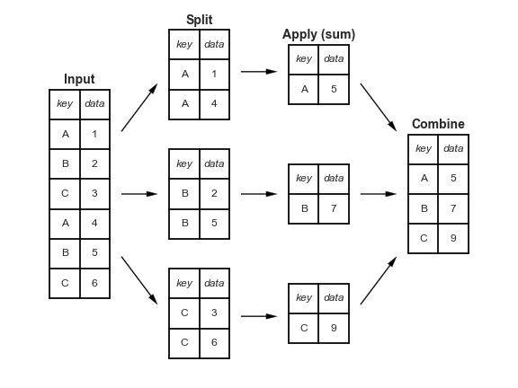
GroupBy: Split, Apply, Combine

Split, apply, combine

In [11]:
df = pd.DataFrame({'key': ['A', 'B', 'C', 'A', 'B', 'C'],
                   'data': range(6)}, columns=['key', 'data'])
df
Out[11]:
key data
0 A 0
1 B 1
2 C 2
3 A 3
4 B 4
5 C 5
In [12]:
df.groupby('key')
Out[12]:
<pandas.core.groupby.DataFrameGroupBy object at 0x117272160>
In [13]:
df.groupby('key').sum()
Out[13]:
data
key
A 3
B 5
C 7

The objeto GroupBy

Indexado por columna

In [14]:
planets.groupby('method')
Out[14]:
<pandas.core.groupby.DataFrameGroupBy object at 0x1172727b8>
In [15]:
planets.groupby('method')['orbital_period']
Out[15]:
<pandas.core.groupby.SeriesGroupBy object at 0x117272da0>
In [16]:
planets.groupby('method')['orbital_period'].median()
Out[16]:
method
Astrometry                         631.180000
Eclipse Timing Variations         4343.500000
Imaging                          27500.000000
Microlensing                      3300.000000
Orbital Brightness Modulation        0.342887
Pulsar Timing                       66.541900
Pulsation Timing Variations       1170.000000
Radial Velocity                    360.200000
Transit                              5.714932
Transit Timing Variations           57.011000
Name: orbital_period, dtype: float64

Iteraciones sobre grupos

In [17]:
for (method, group) in planets.groupby('method'):
    print("{0:30s} shape={1}".format(method, group.shape))
Astrometry                     shape=(2, 6)
Eclipse Timing Variations      shape=(9, 6)
Imaging                        shape=(38, 6)
Microlensing                   shape=(23, 6)
Orbital Brightness Modulation  shape=(3, 6)
Pulsar Timing                  shape=(5, 6)
Pulsation Timing Variations    shape=(1, 6)
Radial Velocity                shape=(553, 6)
Transit                        shape=(397, 6)
Transit Timing Variations      shape=(4, 6)

Métodos de envío (dispactch)

In [18]:
planets.groupby('method')['year'].describe().unstack()
Out[18]:
count mean std min 25% 50% 75% max
method
Astrometry 2.0 2011.500000 2.121320 2010.0 2010.75 2011.5 2012.25 2013.0
Eclipse Timing Variations 9.0 2010.000000 1.414214 2008.0 2009.00 2010.0 2011.00 2012.0
Imaging 38.0 2009.131579 2.781901 2004.0 2008.00 2009.0 2011.00 2013.0
Microlensing 23.0 2009.782609 2.859697 2004.0 2008.00 2010.0 2012.00 2013.0
Orbital Brightness Modulation 3.0 2011.666667 1.154701 2011.0 2011.00 2011.0 2012.00 2013.0
Pulsar Timing 5.0 1998.400000 8.384510 1992.0 1992.00 1994.0 2003.00 2011.0
Pulsation Timing Variations 1.0 2007.000000 NaN 2007.0 2007.00 2007.0 2007.00 2007.0
Radial Velocity 553.0 2007.518987 4.249052 1989.0 2005.00 2009.0 2011.00 2014.0
Transit 397.0 2011.236776 2.077867 2002.0 2010.00 2012.0 2013.00 2014.0
Transit Timing Variations 4.0 2012.500000 1.290994 2011.0 2011.75 2012.5 2013.25 2014.0

Aggregate, filter, transform, apply

In [19]:
rng = np.random.RandomState(0)
df = pd.DataFrame({'key': ['A', 'B', 'C', 'A', 'B', 'C'],
                   'data1': range(6),
                   'data2': rng.randint(0, 10, 6)},
                   columns = ['key', 'data1', 'data2'])
df
Out[19]:
key data1 data2
0 A 0 5
1 B 1 0
2 C 2 3
3 A 3 3
4 B 4 7
5 C 5 9

Agregación

In [20]:
df.groupby('key').aggregate(['min', np.median, max])
Out[20]:
data1 data2
min median max min median max
key
A 0 1.5 3 3 4.0 5
B 1 2.5 4 0 3.5 7
C 2 3.5 5 3 6.0 9
In [21]:
df.groupby('key').aggregate({'data1': 'min',
                             'data2': 'max'})
Out[21]:
data1 data2
key
A 0 5
B 1 7
C 2 9

Filtrado

In [22]:
def filter_func(x):
    return x['data2'].std() > 4

display('df', "df.groupby('key').std()", "df.groupby('key').filter(filter_func)")
Out[22]:

df

key data1 data2
0 A 0 5
1 B 1 0
2 C 2 3
3 A 3 3
4 B 4 7
5 C 5 9

df.groupby('key').std()

data1 data2
key
A 2.12132 1.414214
B 2.12132 4.949747
C 2.12132 4.242641

df.groupby('key').filter(filter_func)

key data1 data2
1 B 1 0
2 C 2 3
4 B 4 7
5 C 5 9

Transformación

In [23]:
df.groupby('key').transform(lambda x: x - x.mean())
Out[23]:
data1 data2
0 -1.5 1.0
1 -1.5 -3.5
2 -1.5 -3.0
3 1.5 -1.0
4 1.5 3.5
5 1.5 3.0

El método apply()

In [24]:
def norm_by_data2(x):
    # x is a DataFrame of group values
    x['data1'] /= x['data2'].sum()
    return x

display('df', "df.groupby('key').apply(norm_by_data2)")
Out[24]:

df

key data1 data2
0 A 0 5
1 B 1 0
2 C 2 3
3 A 3 3
4 B 4 7
5 C 5 9

df.groupby('key').apply(norm_by_data2)

key data1 data2
0 A 0.000000 5
1 B 0.142857 0
2 C 0.166667 3
3 A 0.375000 3
4 B 0.571429 7
5 C 0.416667 9

Especificación de la llave de separación

Usar lista, array, series, or indice como llave para indicar los grupos

In [25]:
L = [0, 1, 0, 1, 2, 0]
display('df', 'df.groupby(L).sum()')
Out[25]:

df

key data1 data2
0 A 0 5
1 B 1 0
2 C 2 3
3 A 3 3
4 B 4 7
5 C 5 9

df.groupby(L).sum()

data1 data2
0 7 17
1 4 3
2 4 7
In [26]:
display('df', "df.groupby(df['key']).sum()")
Out[26]:

df

key data1 data2
0 A 0 5
1 B 1 0
2 C 2 3
3 A 3 3
4 B 4 7
5 C 5 9

df.groupby(df['key']).sum()

data1 data2
key
A 3 8
B 5 7
C 7 12

Usar un diccionario o series como mapeo de los indices para agrupar

In [27]:
df2 = df.set_index('key')
mapping = {'A': 'vowel', 'B': 'consonant', 'C': 'consonant'}
display('df2', 'df2.groupby(mapping).sum()')
Out[27]:

df2

data1 data2
key
A 0 5
B 1 0
C 2 3
A 3 3
B 4 7
C 5 9

df2.groupby(mapping).sum()

data1 data2
consonant 12 19
vowel 3 8

Cualquier función de Python

In [28]:
display('df2', 'df2.groupby(str.lower).mean()')
Out[28]:

df2

data1 data2
key
A 0 5
B 1 0
C 2 3
A 3 3
B 4 7
C 5 9

df2.groupby(str.lower).mean()

data1 data2
a 1.5 4.0
b 2.5 3.5
c 3.5 6.0

Una lista de llaves válidas

In [29]:
df2.groupby([str.lower, mapping]).mean()
Out[29]:
data1 data2
a vowel 1.5 4.0
b consonant 2.5 3.5
c consonant 3.5 6.0

Ejemplo de agrupación

In [30]:
decade = 10 * (planets['year'] // 10)
decade = decade.astype(str) + 's'
decade.name = 'decade'
planets.groupby(['method', decade])['number'].sum().unstack().fillna(0)
Out[30]:
decade 1980s 1990s 2000s 2010s
method
Astrometry 0.0 0.0 0.0 2.0
Eclipse Timing Variations 0.0 0.0 5.0 10.0
Imaging 0.0 0.0 29.0 21.0
Microlensing 0.0 0.0 12.0 15.0
Orbital Brightness Modulation 0.0 0.0 0.0 5.0
Pulsar Timing 0.0 9.0 1.0 1.0
Pulsation Timing Variations 0.0 0.0 1.0 0.0
Radial Velocity 1.0 52.0 475.0 424.0
Transit 0.0 0.0 64.0 712.0
Transit Timing Variations 0.0 0.0 0.0 9.0