< Agregaciones: Min, Max, etc. | Contenido | Comparaciones, máscaras y lógica booleana >

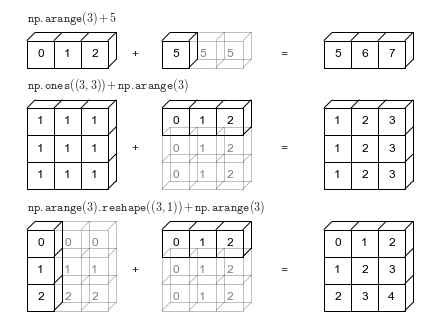
Introducción a Broadcasting¶

In [1]:

import numpy as np

In [2]:

a = np.array([0, 1, 2])
b = np.array([5, 5, 5])
a + b

Out[2]:

array([5, 6, 7])

In [3]:

a + 5

Out[3]:

array([5, 6, 7])

In [4]:

M = np.ones((3, 3))
M

Out[4]:

array([[ 1.,  1.,  1.],
       [ 1.,  1.,  1.],
       [ 1.,  1.,  1.]])

In [5]:

M + a

Out[5]:

array([[ 1.,  2.,  3.],
       [ 1.,  2.,  3.],
       [ 1.,  2.,  3.]])

In [6]:

a = np.arange(3)
b = np.arange(3)[:, np.newaxis]

print(a)
print(b)

[0 1 2]
[[0]
 [1]
 [2]]

In [7]:

a + b

Out[7]:

array([[0, 1, 2],
       [1, 2, 3],
       [2, 3, 4]])

Broadcasting Visual

Reglas del Broadcasting¶

Rule 1: If the two arrays differ in their number of dimensions, the shape of the one with fewer dimensions is padded with ones on its leading (left) side.
Rule 2: If the shape of the two arrays does not match in any dimension, the array with shape equal to 1 in that dimension is stretched to match the other shape.
Rule 3: If in any dimension the sizes disagree and neither is equal to 1, an error is raised.

To make these rules clear, let's consider a few examples in detail.

Broadcasting ejemplo 1¶

In [8]:

M = np.ones((2, 3))
a = np.arange(3)

Let's consider an operation on these two arrays. The shape of the arrays are

M.shape = (2, 3)
a.shape = (3,)

We see by rule 1 that the array a has fewer dimensions, so we pad it on the left with ones:

M.shape -> (2, 3)
a.shape -> (1, 3)

By rule 2, we now see that the first dimension disagrees, so we stretch this dimension to match:

M.shape -> (2, 3)
a.shape -> (2, 3)

The shapes match, and we see that the final shape will be (2, 3):

In [9]:

M + a

Out[9]:

array([[ 1.,  2.,  3.],
       [ 1.,  2.,  3.]])

Broadcasting ejemplo 2¶

In [10]:

a = np.arange(3).reshape((3, 1))
b = np.arange(3)

Again, we'll start by writing out the shape of the arrays:

a.shape = (3, 1)
b.shape = (3,)

Rule 1 says we must pad the shape of b with ones:

a.shape -> (3, 1)
b.shape -> (1, 3)

And rule 2 tells us that we upgrade each of these ones to match the corresponding size of the other array:

a.shape -> (3, 3)
b.shape -> (3, 3)

Because the result matches, these shapes are compatible. We can see this here:

In [11]:

a + b

Out[11]:

array([[0, 1, 2],
       [1, 2, 3],
       [2, 3, 4]])

Broadcasting ejemplo 3¶

In [12]:

M = np.ones((3, 2))
a = np.arange(3)

This is just a slightly different situation than in the first example: the matrix M is transposed. How does this affect the calculation? The shape of the arrays are

M.shape = (3, 2)
a.shape = (3,)

Again, rule 1 tells us that we must pad the shape of a with ones:

M.shape -> (3, 2)
a.shape -> (1, 3)

By rule 2, the first dimension of a is stretched to match that of M:

M.shape -> (3, 2)
a.shape -> (3, 3)

Now we hit rule 3–the final shapes do not match, so these two arrays are incompatible, as we can observe by attempting this operation:

In [13]:

M + a

---------------------------------------------------------------------------
ValueError                                Traceback (most recent call last)
<ipython-input-13-9e16e9f98da6> in <module>()
----> 1 M + a

ValueError: operands could not be broadcast together with shapes (3,2) (3,)

Note the potential confusion here: you could imagine making a and M compatible by, say, padding a's shape with ones on the right rather than the left. But this is not how the broadcasting rules work! That sort of flexibility might be useful in some cases, but it would lead to potential areas of ambiguity. If right-side padding is what you'd like, you can do this explicitly by reshaping the array (we'll use the np.newaxis keyword introduced in The Basics of NumPy Arrays):

In [14]:

a[:, np.newaxis].shape

Out[14]:

(3, 1)

In [15]:

M + a[:, np.newaxis]

Out[15]:

array([[ 1.,  1.],
       [ 2.,  2.],
       [ 3.,  3.]])

Also note that while we've been focusing on the + operator here, these broadcasting rules apply to any binary ufunc. For example, here is the logaddexp(a, b) function, which computes log(exp(a) + exp(b)) with more precision than the naive approach:

In [16]:

np.logaddexp(M, a[:, np.newaxis])

Out[16]:

array([[ 1.31326169,  1.31326169],
       [ 1.69314718,  1.69314718],
       [ 2.31326169,  2.31326169]])

For more information on the many available universal functions, refer to Computation on NumPy Arrays: Universal Functions.

Broadcasting en práctica¶

Centralidad. Subtraer el promedio de un array¶

In [17]:

X = np.random.random((10, 3))

In [18]:

Xmean = X.mean(0)
Xmean

Out[18]:

array([ 0.53514715,  0.66567217,  0.44385899])

In [19]:

X_centered = X - Xmean

In [20]:

X_centered.mean(0)

Out[20]:

array([  2.22044605e-17,  -7.77156117e-17,  -1.66533454e-17])

Graficando una funcion en dos dimensiones¶

In [21]:

# x and y have 50 steps from 0 to 5
x = np.linspace(0, 5, 50)
y = np.linspace(0, 5, 50)[:, np.newaxis]

z = np.sin(x) ** 10 + np.cos(10 + y * x) * np.cos(x)

In [22]:

%matplotlib inline
import matplotlib.pyplot as plt

In [23]:

plt.imshow(z, origin='lower', extent=[0, 5, 0, 5],
           cmap='viridis')
plt.colorbar();

< Agregaciones: Min, Max, etc. | Contenido | Comparaciones, máscaras y lógica booleana >